4.0 Image Gradients and Gradient Filtering

In this class, we will learn about Image Gradients and Gradient Filtering.

 

 

 

 

● Image Edge

2D function Image

We can view an image as a 2D function.

 

 

How can we detect an edge?

What kinds of filter should we use?

 

 

 

● Forward Difference

Forward Difference

We have learned the formula above in high school.

The derivative of a function f at a point x is defined by the limit.

The formula above is the approximation of the derivative when h is small.

This definition is based on the 'forward difference'.

 

 

 

● Central Difference

Central Difference

However, it turns out that using the 'central difference' is more accurate.

 

Then, how do we compute the derivative of a discrete signal?

Discrete Signal

 

 

 

● Sobel Filter

Sobel Filter

The filter above is a derivative filter with some smoothing.

FIlter returns large response on horizontal edges.

The output can be positive or negative.

 

 

 

Approximationo of the derivative of a Gaussian

 

Left one is the original image, and the middle one is a derivative in X direction.

Right one is a derivative in Y direction.

We can visualize negative derivatives or gradients with scaled absolute value.

 

 

 

Then, where does this filter from?

 

 

 

 

● Decomposing the Sobel Filter

Let's decompose the Sobel Filter.

Decomposing the Sobel Filter

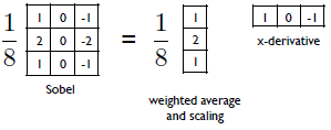
The Sobel Filter is composed of weighted average & scaling, and x-derivative.

 

 

 

The Sobel Filter only returns the x and y edge responses.

 

 

 

● Computing the Image Gradient

How can we compute the image gradient?

 

 

 

① Choose a Derivative Filter

Derivative Filter

 

② Run Filter over Image

 

 

③ Store Image Gradient

 

 

 

 

● Image Gradient

As you can see the pictures above, gradient in x only, has a form of y being 0.

Likewise, gradient in y only, has a form of x being 0.

If we want to consider gradient in both x and y, we should differentiate f with both x and y.

 

 

 

 

* Gradient Direction

Gradient Direction

 

* Gradient Magnitude

Gradient Magnitude

 

 

 

● Common Derivative Filters

① Sobel

Sobel Filter

 

② Scharr

Scharr Filter

 

③ Prewitt

Prewitt Filter

 

④ Roberts

Roberts Filter

 

 

 

 

● Finding edge from signal

 

Intensity Plot

We can also find the edge from the signal by using a derivative filter.

 

 

Derivative Plot

Then we can get a derivative plot.

But derivative filters are sensitive to noise.

 

 

We shouldn't forget to smooth before running derivative filters.

 

 

 

 

 

● Laplace Filter

 

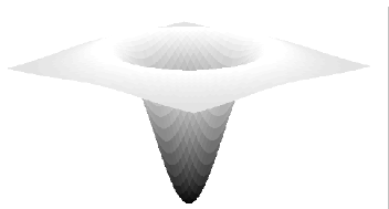
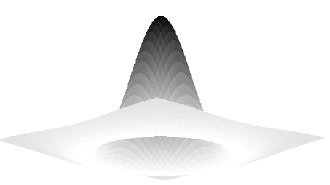
Laplace Filter looks like a straw hat.

 

 

first-order finite difference

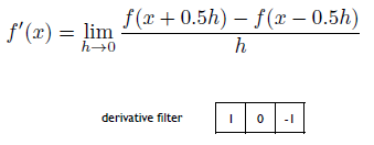
The formula above is the first-order finite difference. We can get derivative filter.

 

 

second-order finite difference

If we apply second-order finite difference above,

we can get Laplace filter like above.

 

 

 

Then what would happen if we apply Laplacian to the intensity plot?

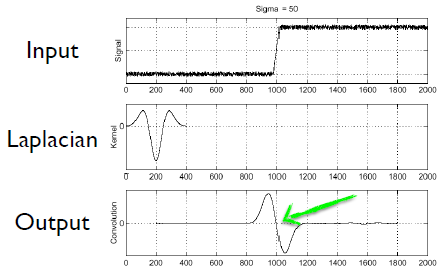
Zero crossings are more accurate at localizing edges.

Second derivative is noisy.

 

 

 

 

 

● 2D Laplace Filter

2D Laplace Filter

 

Laplace Filter

If the Sobel filter approximates the first derivative, the Laplace filter approximates to the second derivative.

 

Laplace Filter and Sobel Filter

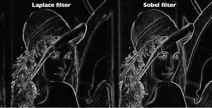
Then what's the difference between Laplace filter and Sobel filter?

 

 

 

Zero crossing

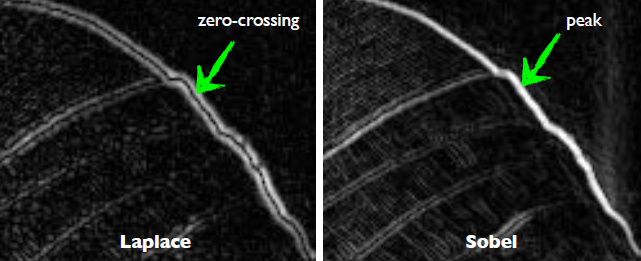
If we look in detail, zero crossings are more accurate at localizing edges.

(but not very convenient)

 

 

 

 

● Summary

 

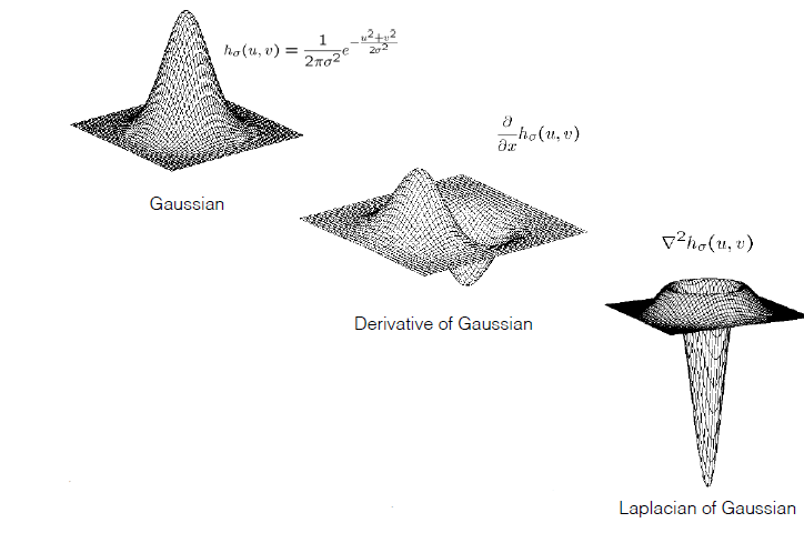
In next class, we will learn about Filtering vs Convolution.